PID Tuning with Relay Feedback (‎Åström–‎Hägglund)

Introduction

The relay feedback method (‎Åström & Hägglund) lets you measure a process’s critical gain $K_u$ and ultimate period $T_u$ without pushing the plant into sustained oscillations with a proportional controller. Instead, you close the loop with an on–off relay and record the limit-cycle amplitude $a$ that results.

Compared to PID tuning from an open-loop step response, relay feedback is:

• Safer: the amplitude of oscillation is bounded by relay hysteresis.
• Online: can be performed while the process is under closed-loop control.
• Model-free: does not require fitting $K$, $T$, $L$ first.

Prerequisites

• Familiarity with FOLPD models and basic PID tuning concepts (see Getting Started)
• python-control ≥ 0.10.1 and scipy
• The control_utils.py toolkit used in Getting Started

---

Theory

Relay in the Feedback Loop

Replace the PID controller with a relay that switches between $+d$ and $-d$ based on the sign of error:

$$u(t) = d \cdot \text{sgn}\bigl(r(t) - y(t)\bigr)$$

For a low-pass process plus time-delay, the relay induces a stable limit cycle. By describing-function analysis, the first harmonic of the relay output has amplitude:

$$u_1 = \frac{4d}{\pi}$$

At the ultimate frequency $\omega_u = 2\pi / T_u$, the loop gain is $-1$, so the plant magnitude at $\omega_u$ satisfies:

$$\frac{4d}{\pi} \cdot \bigl|G(j\omega_u)\bigr| = a \quad\Rightarrow\quad K_u = \frac{1}{\bigl|G(j\omega_u)\bigr|} = \frac{4d}{\pi a}$$

Ziegler–Nichols Frequency-Domain Rules

Once $(K_u, T_u)$ are known, the ZN tuning rules are (PID form):

Parameter	Formula
$K_p$	$0.60 \, K_u$
$T_i$	$0.50 \, T_u$
$T_d$	$0.125 \, T_u$

Which translate to standard gains:

$$K_i = \frac{K_p}{T_i} = \frac{1.2 \, K_u}{T_u}, \qquad K_d = K_p \, T_d = 0.075 \, K_u \, T_u$$

---

Experiment Setup

The Process

We use a standard FOLPD plant:

$$G(s) = \frac{20 \, e^{-s}}{10s + 1}$$

Parameters: $K=20$, $T=10\,\text{s}$, $L=1\,\text{s}$.

Relay Controller

In python-control≥0.10, a static nonlinear controller is built with ct.nlsys:

import numpy as np
import control as ct

def relay_output(t, xc, uc, params):
    e = uc[0]
    d = params['b']           # relay amplitude
    return [np.sign(e) * d]

relay = ct.nlsys(
    lambda t, xc, uc, params: [0],   # no internal states
    relay_output,
    inputs=('e'), outputs=('u'),
    states=0, params={'b': 5.0},
    name='relay', dt=0
)

# Summing junction: e = r - y
sumblk = ct.summing_junction(inputs=['r', '-y'], output='e')

# Close the loop
T_ry = ct.interconnect(
    [G, relay, sumblk],
    inplist='r', outlist='y'
)

Simulation

A unit step reference ($r=1$) forces the relay to switch continuously once the transients decay:

T_sim, dt = 200, 0.01
timepts = np.arange(0, T_sim, dt)
r = np.ones(len(timepts))

resp_y = ct.input_output_response(T_ry, timepts, r)

---

Measuring the Limit Cycle

After discarding the initial transient, identify peaks and valleys of the steady-state oscillation:

from scipy.signal import find_peaks

idx_start = int(120 / dt)           # after t = 120 s
y_ss = np.asarray(resp_y.outputs[idx_start:]).flatten()

mean_y = float(np.mean(y_ss))
peaks, _ = find_peaks(y_ss, height=mean_y, distance=int(2.0 / dt))
valleys, _ = find_peaks(-y_ss, height=-mean_y, distance=int(2.0 / dt))

# Oscillation amplitude
a = (np.mean(y_ss[peaks]) - np.mean(y_ss[valleys])) / 2.0

# Ultimate period
periods = [
    resp_y.time[peaks[i+1]] - resp_y.time[peaks[i]]
    for i in range(len(peaks) - 1)
]
Tu = float(np.mean(periods))

For this example, we measure:

Quantity	Value	Units
Relay amplitude $d$	5	—
Limit-cycle amplitude $a$	8.60	process units
Ultimate period $T_u$	3.82	s
Ultimate gain $K_u$	0.74	—

Verification: ct.margin(G) reports a gain margin of $0.818$ at $\omega = 1.63\,\text{rad/s}$ ($T_u = 2\pi/1.63 \approx 3.85\,\text{s}$). The relay estimate is within $\sim 10\%$ of the true linear-system value, which is typical for describing-function approximations.

Experimental Waveform

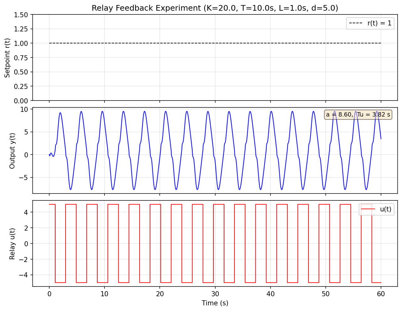
The limit cycle establishes within ~20 s after the step; the steady-state amplitude $a$ and period $T_u$ are read from this waveform. The first 120 s are discarded when computing the average to avoid Pade startup transients.

---

Computing PID Gains

Plug the measured $(K_u, T_u)$ into the ZN frequency-domain formulas:

Ku = 4 * d / (np.pi * a)    # ≈ 0.74
Tu = 3.82

Kp = 0.60 * Ku              # ≈ 0.444
Ki = 1.2 * Ku / Tu          # ≈ 0.233
Kd = 0.075 * Ku * Tu        # ≈ 0.212

---

Comparison: Three ZN Frequency-Domain Variants

The Wikipedia Ziegler–Nichols method page lists several PID variants based on the same $(K_u, T_u)$ data. Below we focus on the three most commonly used forms: Classic, Some overshoot, and No overshoot.

Two Equivalent PID Representations

PID controllers can be written using either time-constant form $(K_p, T_i, T_d)$ or standard gain form $(K_p, K_i, K_d)$. Both are equivalent—choose whichever matches your control-system implementation.

Time-constant form (ISA/PID standard):

$$u(t) = K_p \left[ e(t) + \frac{1}{T_i} \int_0^t e(\tau)\,d\tau + T_d \frac{de}{dt} \right]$$

Standard gain form:

$$u(t) = K_p \, e(t) + K_i \int_0^t e(\tau)\,d\tau + K_d \frac{de}{dt}$$

Conversion formulas:

$$K_i = \frac{K_p}{T_i}, \qquad K_d = K_p \, T_d$$ $$T_i = \frac{K_p}{K_i}, \qquad T_d = \frac{K_d}{K_p}$$

ZN Formulas (Time-Constant Form)

Variant	$K_p$	$T_i$	$T_d$
Classic PID	$0.60 \, K_u$	$0.50 \, T_u$	$0.125 \, T_u$
Some overshoot	$0.333 \, K_u$	$0.50 \, T_u$	$0.333 \, T_u$
No overshoot	$0.20 \, K_u$	$0.50 \, T_u$	$0.333 \, T_u$

Key insight: all three variants share the same integral time $T_i = 0.5 T_u$ and integral gain $K_i = K_p/T_i$. The “some overshoot” and “no overshoot” variants reduce $K_p$ (less proportional action) and increase $T_d$ (more derivative time constant) relative to Classic — but because $K_d = K_p T_d$, the resulting standard derivative gain is higher for “some overshoot” but paradoxically lower for “no overshoot”.

Standard Gains for This Plant

From $K_u \approx 0.74$ and $T_u \approx 3.82$ s:

Method	$K_p$	$T_i$ (s)	$T_d$ (s)	$K_i$	$K_d$
Classic	0.444	1.91	0.478	0.233	0.212
Some overshoot	0.247	1.91	1.273	0.129	0.314
No overshoot	0.148	1.91	1.273	0.078	0.189

Notice: “Some overshoot” achieves the strongest derivative action ($K_d = 0.314$) because its moderately low $K_p$ is multiplied by the maximum $T_d$. Conversely, “No overshoot” drops $K_p$ so far that $K_d = 0.189$ ends up weaker than Classic ($K_d = 0.212$). This explains the counterintuitive simulation result.

---

Response Comparison

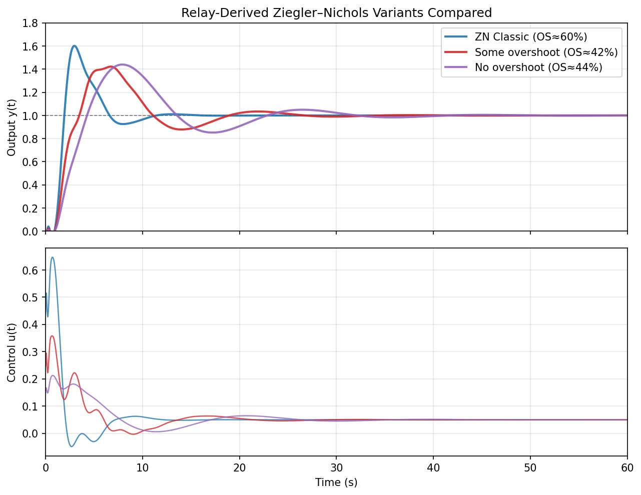
Closed-Loop Performance

All controllers use the same PIDController implementation (anti-windup, derivative-on-measurement, derivative filtering) in discrete time:

Method	Overshoot	Peak Time	Settling (±2%)	IAE	Notes
Classic	≈ 60%	3.0 s	~11 s	3.2	Quarter-wave decay; fast but rings
Some overshoot	≈ 42%	6.7 s	~24 s	4.8	Reduced aggressiveness vs. Classic
No overshoot	≈ 44%	7.9 s	~30 s	6.3	Most conservative rule; still nonzero OS

Understanding the names: “Some overshoot” and “No overshoot” are historical names for these ZN modifications — they indicate the rules are tuned to reduce overshoot compared to the Classic quarter-wave target, but they do not guarantee low overshoot on every process. On plants with significant time delay (like our example with $L/T = 0.1$), these rules still produce substantial overshoot because the fixed structure of ZN rules does not explicitly compensate for phase lag.

For reference: the getting-started tutorial shows similar results — ZN-tuned loops typically show 60–90% overshoot on FOLPD processes with $L/T \approx 0.1–0.2$. Ziegler and Nichols designed these rules for “quarter-wave decay” (aggressive, responsive control), not tight damping. The “some overshoot” and “no overshoot” variants lower $K_p$ and raise $T_d$ relative to Classic, but the effect is modest; true low-overshoot tuning requires model-based methods (IMC) or iterative refinement.

Observations:

• Classic gives the fastest rise but heaviest overshoot (~60%). This is the traditional quarter-wave-decay target — aggressive by design.
• Some overshoot reduces proportional gain and raises derivative time compared to Classic, producing a slower but somewhat smoother response. The overshoot drops from ~60% to ~42%.
• No overshoot uses the lowest proportional gain and a moderate derivative time. Despite the name, overshoot remains ~44% because the derivative gain ($K_d = 0.067 K_u T_u$) is actually lower than “Some overshoot” ($K_d = 0.111 K_u T_u$). This is counterintuitive: one might expect “No overshoot” to have the strongest derivative damping, but the Wikipedia-quoted rule does not. A purely delay-dominant process benefits more from high derivative action; reducing $K_p$ without sufficient $K_d$ can leave the oscillatory mode underdamped.

Rule	What it actually does	Result on this plant
Classic	Maximum $K_p$, minimum $T_d$	Fastest, ~60% OS
Some overshoot	Moderate $K_p$, maximum $T_d$	Moderate, ~42% OS
No overshoot	Minimum $K_p$, moderate $T_d$	Slowest, ~44% OS

Key finding: on this plant (large process gain $K=20$ with $L/T = 0.1$), “Some overshoot” actually achieves the lowest peak overshoot, not “No overshoot”. The name “No overshoot” reflects the intended design philosophy (even more conservative than “Some overshoot”), but it does not translate to guaranteed low overshoot on all processes.

When to use each variant

	Classic	Some overshoot	No overshoot
Intended use	Quarter-wave decay	Moderately damped	Most conservative
Rise time	Fastest	Moderate	Slowest
When to use	Tolerant processes, fast tracking	Balanced speed / smoothness	Most conservative starting point
Actual OS on this plant	~60%	~42%	~44%
Tip	Expect aggressive tuning	Good first refinement	Lower gains, but not guaranteed low OS

---

Practical Tips

Tip	Why It Matters
Discard ≥ 5 time constants before measuring $a$ and $T_u$	Non-stationary startup from Pade approximation corrupts early cycles
Choose $d$ so that $a \gg$ measurement noise	Low SNR makes peak detection unreliable
Add small hysteresis $\varepsilon$ to the relay	Prevents chattering from zero-crossing noise
For integrating processes, bias the relay	Prevents output drift while still exciting the critical mode

---

Extensions

1. Modified relay methods: a relay with hysteresis ($\varepsilon$) lets you target phase margins directly rather than just the ultimate point. See Åström & Hägglund (2006) §4.2.
2. On-line re-tuning: run the relay experiment briefly, compute gains, then switch back to PID automatically — no manual intervention.
3. Model-based refinement: if you also want a FOLPD model, fit $K_u$ and $T_u$ back to $(K, T, L)$ and then apply IMC rules for explicit robustness–performance trade-off.

---

Reproducibility

The complete plotting script used to generate the figures in this tutorial:

• Download generate_relay_feedback_plots.py (Python script, ~400 lines)

Dependencies: python-control ≥ 0.10.1, scipy, matplotlib, and the local control_utils.py module. Run it directly to reproduce all figures. The script is also available in the python-control GitHub repository.

---

References

1. Åström, K.J., & Hägglund, T. (2006). Advanced PID Control. ISA.

---

Try It Yourself

• Experiment with the relay amplitude $d$ (larger → bigger oscillation → easier to measure, but more disturbance)
• Try all three ZN variants on your own process and compare the response smoothness
• Return to the Getting Started with PID Tuning tutorial for open-loop step-response methods